In this post we are going to play with pyextremes a python library that does everything (and more) I have been talking about the two previous posts. After a bit of EDA, we are going to fit use BM and POT to compute the return values – could be interesting to know what magnitude to expect at a given horizon, no?
\(m\)-years return values/levels are the “high quantile for which the probability that the annual maximum exceeds this quantile is \(1/m\)” – see 100-year flood (wiki).
Setup and data - Earthquakes in CA
Setup
A bit of setup first…
!pip3.8 install -q -U emcee folium pyextremes statsmodelsimport pandas as pd
import numpy as np
%matplotlib inline
import matplotlib as mpl
from matplotlib import pylab as plt
import matplotlib.dates as mdates
import seaborn as sns
sns.set(rc={'figure.figsize':(18,6)})
sns.set_style("ticks")
cmap = plt.get_cmap('plasma')
import statsmodels.api as sm
from pyextremes import EVA, __version__
import pyextremes
from pyextremes.plotting import (
plot_extremes,
plot_trace,
plot_corner,
)
vmin=3.0
vmax=9.0
print("pyextremes", __version__)pyextremes 2.2.1Data
Data are from the Northern California Earthquake Data Center (NCEDC).
- Waldhauser, F. and D.P. Schaff, Large-scale relocation of two decades of Northern California seismicity using cross-correlation and double-difference methods, J. Geophys. Res.,113, B08311, doi:10.1029/2007JB005479, 2008.
- Waldhauser, F., Near-real-time double-difference event location using long-term seismic archives, with application to Northern California, Bull. Seism. Soc. Am., 99, 2736-2848, doi:10.1785/0120080294, 2009.
Go here if you want to download them.
df_ = pd.read_csv('ncedc.csv')
df_| time | latitude | longitude | magnitude | magType | … | source | eventID | |
|---|---|---|---|---|---|---|---|---|
| 0 | 1967/08/22 08:29:47.47 | 36.40050 | -120.98650 | 3.00 | Mx | … | NCSN | 1001120 |
| 1 | 1967/08/26 10:35:05.61 | 36.53867 | -121.16033 | 3.30 | Mx | … | NCSN | 1001154 |
| 2 | 1967/08/27 13:20:08.75 | 36.51083 | -121.14500 | 3.60 | Mx | … | NCSN | 1001166 |
| 3 | 1968/01/12 22:19:10.35 | 36.64533 | -121.24966 | 3.00 | ML | … | NCSN | 1001353 |
| 4 | 1968/02/09 13:42:37.05 | 37.15267 | -121.54483 | 3.00 | ML | … | NCSN | 1001402 |
| … | … | … | … | … | … | … | … | … |
| 18330 | 2020/12/27 14:44:40.09 | 39.50583 | -122.01767 | 3.86 | Mw | … | NCSN | 73503450 |
| 18331 | 2020/12/27 19:05:47.53 | 36.84417 | -121.57484 | 3.19 | ML | … | NCSN | 73503535 |
| 18332 | 2020/12/30 08:30:22.09 | 36.60500 | -121.20883 | 3.10 | ML | … | NCSN | 73504420 |
| 18333 | 2020/12/31 04:22:03.38 | 38.83883 | -122.82317 | 3.63 | Mw | … | NCSN | 73504795 |
| 18334 | 2020/12/31 13:41:59.04 | 37.79950 | -122.59367 | 3.33 | ML | … | NCSN | 73505175 |
18335 rows × 12 columns
magTypeColors = sns.color_palette("hls", 8)
palette = {
    'ML': magTypeColors[0],
    'Md': magTypeColors[1],
    'Mh': magTypeColors[2],
    'Mw': magTypeColors[3],
    'Mx': magTypeColors[4],
    'Unk': magTypeColors[5],
}
sns.histplot(data=df_.sort_values(by='magType'),
             x='magnitude',
             hue='magType',
             bins=20,
             multiple='stack',
             palette=palette)
sns.despine(left=True)
plt.show()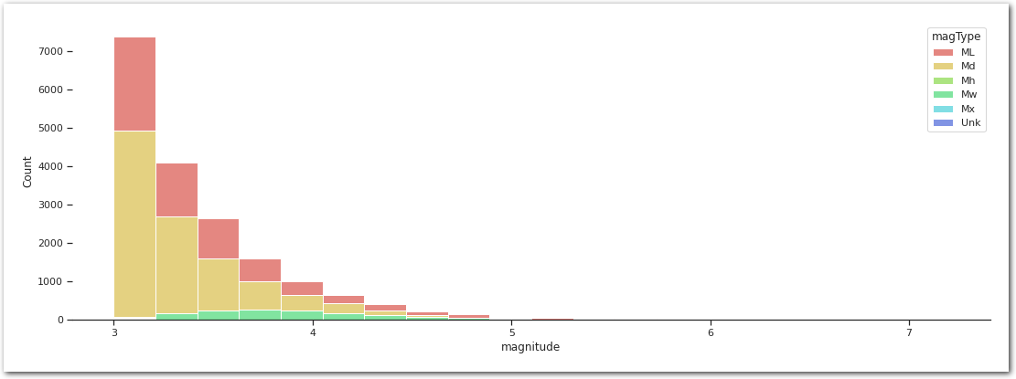
And more specifically above 5.
sns.histplot(data=df_[df_['magnitude'] > 5].sort_values(by='magType'),
             x='magnitude',
             hue='magType',
             bins=20,
             multiple='stack',
             palette=palette)
sns.despine(left=True)
plt.show()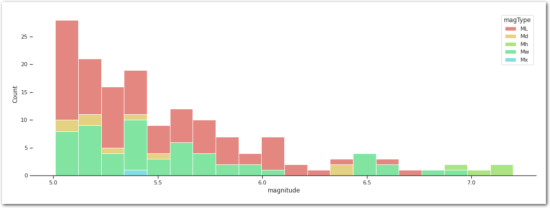
The magniture are based on different scales.
df_.groupby(by='magType').size().to_frame('count')| magType | count |
|---|---|
| ML | 6513 |
| Md | 10307 |
| Mh | 12 |
| Mw | 1456 |
| Mx | 46 |
| Unk | 1 |
We will stick to only one scale as mapping on to each other seems to be difficult. They basically measure different things… – See USGS - what-are-different-magnitude-scales.
We pick moment magnitude (Mw) scale as “[it is] based on the concept of seismic moment, is uniformly applicable to all sizes of earthquakes but is more difficult to compute than the other types” – See magnitude. Other scales are not covering the entire range of eathquakes creating truncated data. Note that this could introduce a selection bias as we are not sure why a particular events is using one scale or another.
df__ = df_[(df_['magType'] == 'Mw')]
df__.groupby(by='magType').size()
Mw 1456df_all = df__[['time', 'latitude', 'longitude', 'magnitude']].copy()
df_all.rename({'magnitude': 'value',
'time': 'obs'}, inplace=True, axis=1)
df_all = df_all.dropna(axis=0)
df_all = df_all.set_index(pd.DatetimeIndex(df_all['obs'])).drop('obs', axis=1)
df_all.head()| obs | latitude | longitude | value |
|---|---|---|---|
| 1992-04-26 07:41:40.090 | 40.43250 | -124.56600 | 6.45 |
| 1992-04-26 11:18:25.980 | 40.38283 | -124.55500 | 6.57 |
| 1992-09-19 23:04:46.830 | 38.86000 | -122.79183 | 4.47 |
| 1993-01-16 06:29:35.010 | 37.01833 | -121.46317 | 4.91 |
| 1993-01-18 23:27:10.610 | 38.84250 | -122.77800 | 3.92 |
sns.histplot(data=df_all, x='value', bins=20, color=palette['Mw'])
sns.despine(left=True)
plt.show()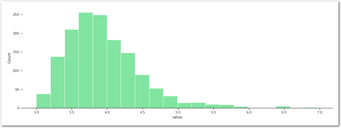
The data we are looking at cover the following time interval:
pd.DataFrame.from_dict(data={'min': [min(df_all.index)],
                             'max': [max(df_all.index)]},
                       orient='index',
columns=['obs'])| obs | |
|---|---|
| min | 1992-04-26 07:41:40.090 |
| max | 2020-12-31 04:22:03.380 |
and range as follows:
pd.DataFrame(df_all['value'].describe())| value | |
|---|---|
| count | 1456.000000 |
| mean | 3.933427 |
| std | 0.535629 |
| min | 3.000000 |
| 25% | 3.560000 |
| 50% | 3.850000 |
| 75% | 4.200000 |
| max | 6.980000 |
The biggest earthquake in CA (in this dataset and using this scale…) are:
df_all.sort_values('value', ascending=False) \
      .nlargest(columns=['value'], n=10) \
      .style.background_gradient(subset=['value'],
                                 cmap=cmap,
                                 vmin=vmin,
vmax=vmax)| obs | latitude | longitude | value |
|---|---|---|---|
| 2005-06-15 02:50:51.330000 | 41.232670 | -125.986340 | 6.980000 |
| 2014-03-10 05:18:13.430000 | 40.828670 | -125.133830 | 6.800000 |
| 1995-02-19 04:03:14.940000 | 40.591840 | -125.756670 | 6.600000 |
| 1992-04-26 11:18:25.980000 | 40.382830 | -124.555000 | 6.570000 |
| 2003-12-22 19:15:56.240000 | 35.700500 | -121.100500 | 6.500000 |
| 2010-01-10 00:27:39.320000 | 40.652000 | -124.692500 | 6.500000 |
| 1992-04-26 07:41:40.090000 | 40.432500 | -124.566000 | 6.450000 |
| 2020-05-15 11:03:26.400000 | 38.216170 | -117.844330 | 6.440000 |
| 2014-08-24 10:20:44.070000 | 38.215170 | -122.312330 | 6.020000 |
| 2004-09-28 17:15:24.250000 | 35.818160 | -120.366000 | 5.970000 |
import folium

def transparent(r, g, b, a, alpha=None):
    if alpha is None:
        return (r, g, b, a)
    return (r, g, b, alpha)
def rgb2hex(r, g, b, a=None):
    if a is None:
        return "#{:02x}{:02x}{:02x}".format(int(r*255),
                                            int(g*255),
                                            int(b*255))
    else:
        return "#{:02x}{:02x}{:02x}{:02x}".format(int(r*255),
                                                  int(g*255),
                                                  int(b*255),
                                                  int(a*255))

m = folium.Map(location=[df_all['latitude'].mean(),
                         df_all['longitude'].mean()],
                         tiles="Stamen Terrain", zoom_start=6)

def add_to_map(row):
    folium.Circle(
        radius=100*row['value'],
        location=[row['latitude'], row['longitude']],
        popup="{obs} {value}".format(obs=row.name,
                                     value=row['value']),
        color=rgb2hex(*transparent(*cmap((row['value']-vmin)/(vmax - vmin)),
                                   alpha=0.5)),
        fill=True,
    ).add_to(m)

df_all.apply(add_to_map, axis=1)

m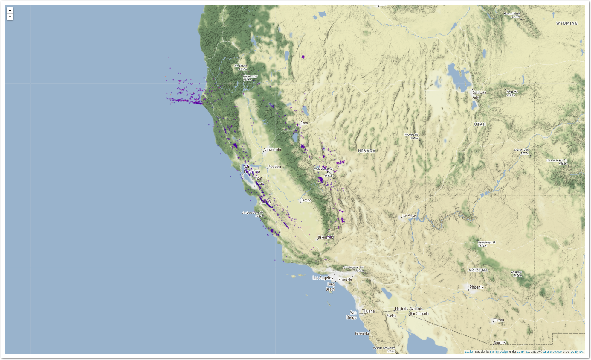
from matplotlib.dates import YearLocator, DateFormatter

sns.scatterplot(data=df_all, x='obs', y='value',
                marker='.', palette=cmap, hue='value',
                hue_norm=(vmin, vmax), s=150, alpha=0.9)
ax = plt.gca()
ax.xaxis.set_major_locator(YearLocator(2))
ax.xaxis.set_major_formatter(DateFormatter('%Y'))
sns.despine(left=True)
plt.show()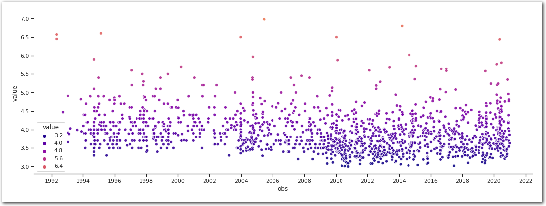
The scale (Mw) seems to have been used throughout the period we are looking at.
data_df = df_all.groupby(by='obs')['value'].max()
data_df.index = pd.to_datetime(data_df.index)
How independent are these events?
sm.graphics.tsa.plot_acf(data_df, lags=20)
sns.despine(left=True)
plt.show()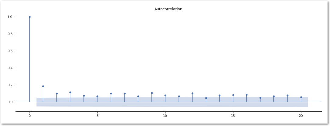
There is a bit of autocorrelation. Not completely surprising as “Aftershocks can continue over a period of weeks, months, or years.” USGS glossary. To remove that we are going look at the max in 1-week windows. It is not perfect as aftershocks can span longer than that and there is no guarantee that all the aftershocks are going to fall in the same buckets. Let see how it does.
data_df_ = data_df.resample('1W').max().dropna()
sm.graphics.tsa.plot_acf(data_df_.squeeze(), lags=20)
sns.despine(left=True)
plt.show()
Looking better.
sns.scatterplot(data=data_df_.to_frame('value'), x='obs', y='value', marker='.', palette=cmap, hue='value', hue_norm=(vmin, vmax), s=150, alpha=0.9)
ax = plt.gca()
ax.xaxis.set_major_locator(YearLocator(2))
ax.xaxis.set_major_formatter(DateFormatter('%Y'))
sns.despine(left=True)
plt.show()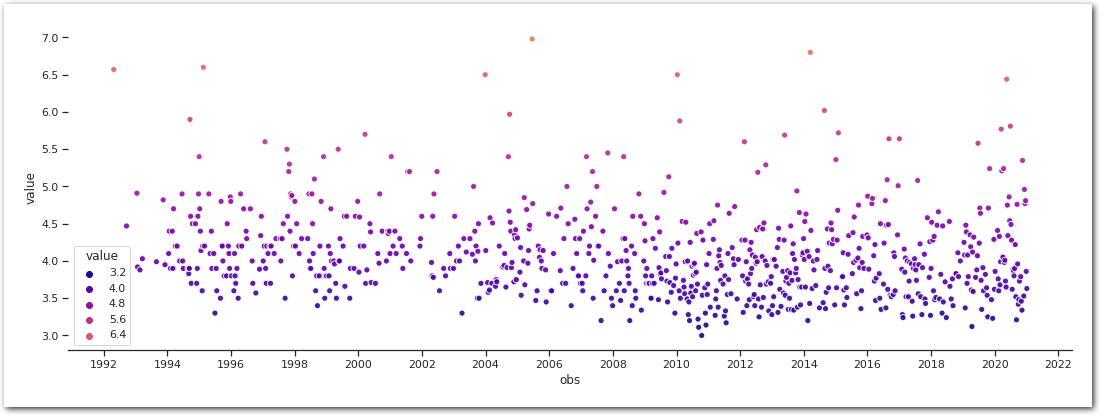
Let’s put the data in the form pyextremes expect them.
data=data_df_.to_frame('value').squeeze()
data
obs
1992-04-26 6.57
1992-09-20 4.47
1993-01-17 4.91
1993-01-24 3.92
1993-02-21 3.88
...
2020-12-06 4.96
2020-12-13 4.77
2020-12-20 4.81
2020-12-27 3.86
2021-01-03 3.63
Name: value, Length: 777, dtype: float64BM model
model = EVA(data=data)
model
Univariate Extreme Value Analysis
===========================================================================
Source Data
---------------------------------------------------------------------------
Data label: value Size: 777
Start: April 1992 End: January 2021
===========================================================================
Extreme Values
---------------------------------------------------------------------------
Extreme values have not been extracted
===========================================================================
Model
---------------------------------------------------------------------------
Model has not been fit to the extremes
===========================================================================model.get_extremes(
method="BM",
extremes_type="high",
block_size="365.2425D",
errors="ignore",
)
model Univariate Extreme Value Analysis
===========================================================================
Source Data
---------------------------------------------------------------------------
Data label: value Size: 777
Start: April 1992 End: January 2021
===========================================================================
Extreme Values
---------------------------------------------------------------------------
Count: 29 Extraction method: BM
Type: high Block size: 365 days 05:49:12
===========================================================================
Model
---------------------------------------------------------------------------
Model has not been fit to the extremes
===========================================================================model.plot_extremes()
sns.despine(left=True)
plt.show()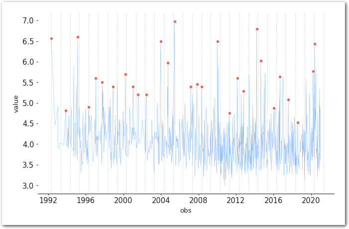
MLE
model.fit_model()
model
Univariate Extreme Value Analysis
===========================================================================
Source Data
---------------------------------------------------------------------------
Data label: value Size: 777
Start: April 1992 End: January 2021
===========================================================================
Extreme Values
---------------------------------------------------------------------------
Count: 29 Extraction method: BM
Type: high Block size: 365 days 05:49:12
===========================================================================
Model
---------------------------------------------------------------------------
Model: MLE Distribution: gumbel_r
Log-likelihood: -28.048 AIC: 60.558
---------------------------------------------------------------------------
Free parameters: loc=5.340 Fixed parameters: All parameters are free
scale=0.550
===========================================================================model.plot_diagnostic(alpha=0.95)
sns.despine(left=True)
plt.show()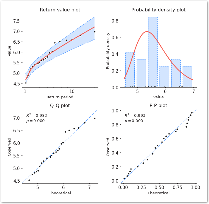
model.plot_return_values(
    return_period=np.logspace(0.01, 2, 100),
    return_period_size="365.2425D",
    alpha=0.95,
)
sns.despine(left=True)
plt.show()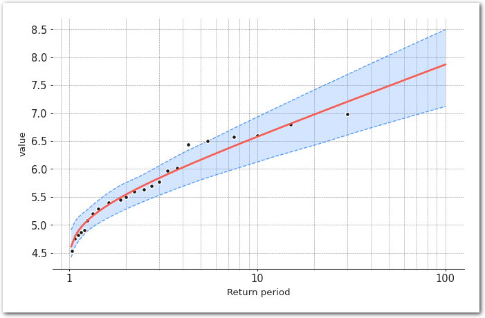
summary_bm_mle = model.get_summary(
    return_period=[2, 5, 10, 25, 50, 100],
    alpha=0.95,
    n_samples=1000,
)
summary_bm_mle.style.background_gradient(cmap=cmap, vmin=vmin, vmax=vmax)| return period | return value | lower ci | upper ci |
|---|---|---|---|
| 2.0 | 5.541965 | 5.327484 | 5.777972 |
| 5.0 | 6.165502 | 5.836295 | 6.472050 |
| 10.0 | 6.578338 | 6.165001 | 6.960001 |
| 25.0 | 7.099957 | 6.576074 | 7.581792 |
| 50.0 | 7.486924 | 6.863262 | 8.037220 |
| 100.0 | 7.871033 | 7.156755 | 8.490038 |
MCMC
The library also supports fitting the distribution using a Bayesian approach. Wont go over this here. Check the tutorials that come with it.
POT
POT requires to select a threshold. A method to do that is to apply the fit the GPD for a range of thresholds and look at the stability of its parameters. This is what the following does:
pyextremes.plot_parameter_stability(ts=data, thresholds=np.linspace(4, 6, 50))
sns.despine(left=True)
plt.show()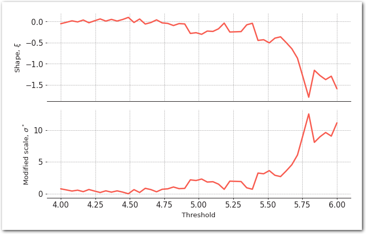
We then pick a threshold in the range where the scale and shape parameters of the GPD are stable.
threshold = 4.25model = EVA(data=data)
model Univariate Extreme Value Analysis
===========================================================================
Source Data
---------------------------------------------------------------------------
Data label: value Size: 777
Start: April 1992 End: January 2021
===========================================================================
Extreme Values
---------------------------------------------------------------------------
Extreme values have not been extracted
===========================================================================
Model
---------------------------------------------------------------------------
Model has not been fit to the extremes
===========================================================================sns.histplot(data=data[data>threshold], bins=20)
sns.despine(left=True)
plt.show()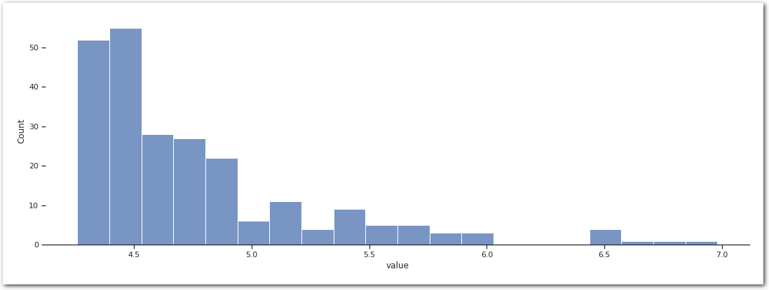
model.get_extremes(
    method="POT",
    extremes_type="high",
    threshold=threshold)
model
Univariate Extreme Value Analysis
===========================================================================
Source Data
---------------------------------------------------------------------------
Data label: value Size: 777
Start: April 1992 End: January 2021
===========================================================================
Extreme Values
---------------------------------------------------------------------------
Count: 237 Extraction method: POT
Type: high Threshold: 4.25
===========================================================================
Model
---------------------------------------------------------------------------
Model has not been fit to the extremes
===========================================================================model.plot_extremes()
sns.despine(left=True)
plt.show()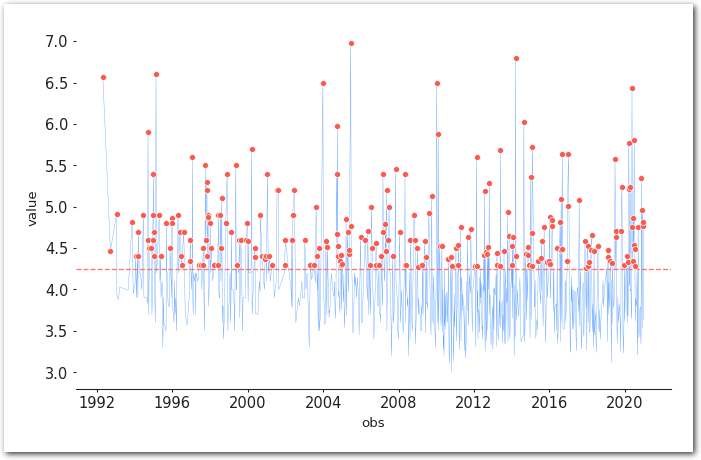
model.fit_model()
model
Univariate Extreme Value Analysis
===========================================================================
Source Data
---------------------------------------------------------------------------
Data label: value Size: 777
Start: April 1992 End: January 2021
===========================================================================
Extreme Values
---------------------------------------------------------------------------
Count: 237 Extraction method: POT
Type: high Threshold: 4.25
===========================================================================
Model
---------------------------------------------------------------------------
Model: MLE Distribution: expon
Log-likelihood: -77.084 AIC: 156.185
---------------------------------------------------------------------------
Free parameters: scale=0.509 Fixed parameters: floc=4.250
===========================================================================model.plot_diagnostic(alpha=0.95)
sns.despine(left=True)
plt.show()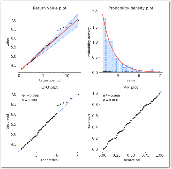
model.plot_return_values(
    return_period=np.logspace(0.01, 2, 100),
    return_period_size="365.2425D",
    alpha=0.95,
)
sns.despine(left=True)
plt.show()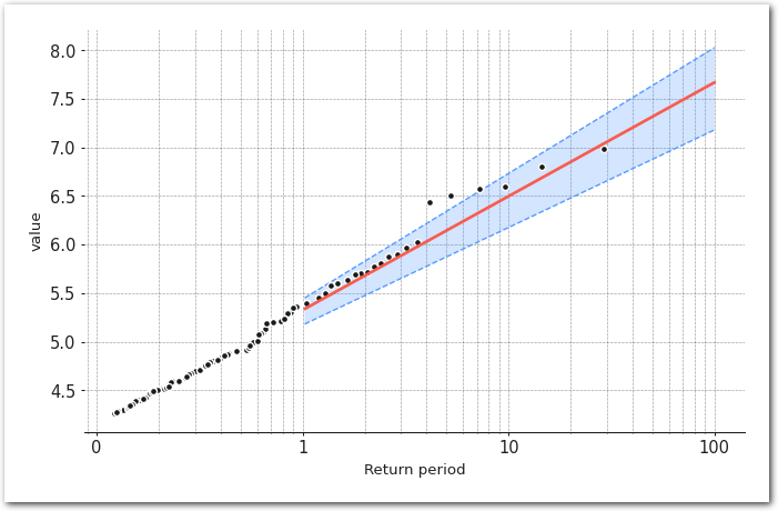
summary_pot_mle = model.get_summary(
    return_period=[2, 5, 10, 25, 50, 100],
    alpha=0.95,
    n_samples=1000,
)
summary_pot_mle.style.background_gradient(cmap=cmap, vmin=vmin, vmax=vmax)| return period | return value | lower ci | upper ci |
|---|---|---|---|
| 2.0 | 5.678355 | 5.508168 | 5.870555 |
| 5.0 | 6.145006 | 5.919218 | 6.399999 |
| 10.0 | 6.498014 | 6.230166 | 6.800508 |
| 25.0 | 6.964665 | 6.641216 | 7.329952 |
| 50.0 | 7.317673 | 6.952163 | 7.730461 |
| 100.0 | 7.670680 | 7.263111 | 8.130970 |
Comparison
Let’s compare what both methods.
df_bm = summary_bm_mle
df_pot = summary_pot_mle
# bm
plt.errorbar(df_bm.index,
             df_bm['return value'],
             yerr=[df_bm['return value'] - df_bm['lower ci'],
                   df_bm['upper ci'] - df_bm['return value']],
             fmt='-ob', label='return value (bm)');
plt.fill_between(df_bm.index,
                 df_bm['lower ci'],
                 df_bm['upper ci'],
                 color='b',
                 alpha=0.2)
# pot
plt.errorbar(df_pot.index,
             df_pot['return value'],
             yerr=[df_pot['return value'] - df_pot['lower ci'],
                   df_pot['upper ci'] - df_pot['return value']],
             fmt='-or',
             label='return value (pot)');
plt.fill_between(df_pot.index,
                 df_pot['lower ci'],
                 df_pot['upper ci'],
                 color='r',
                 alpha=0.2)
plt.grid(True, which="both", linestyle='--', linewidth=1)
plt.gca().set_xscale('log')
plt.title('global earthquakes - return values - bm and pot 95% CIs')
plt.legend()
sns.despine(left=True)
plt.show()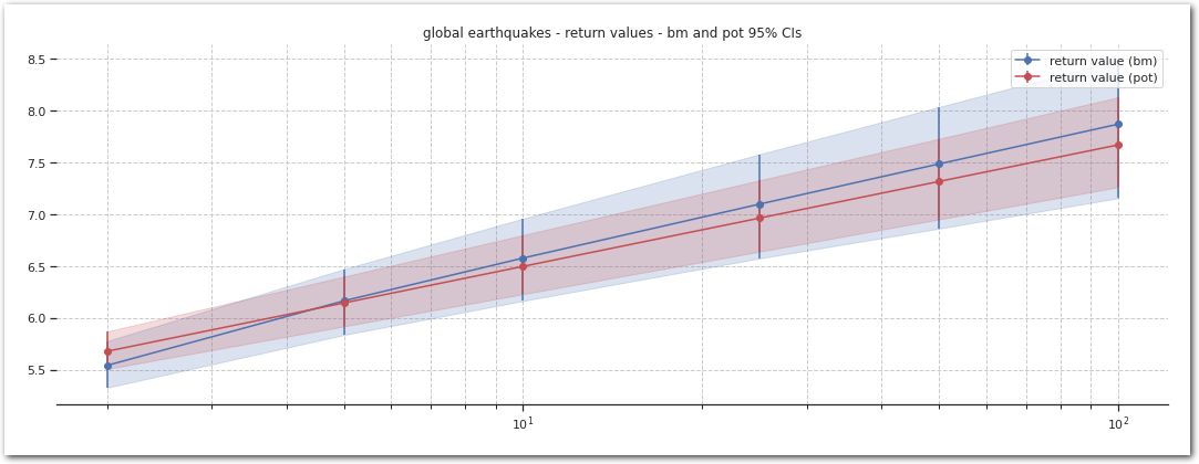
pd.concat([summary_bm_mle, summary_pot_mle],
          axis=1,
          keys=['bm', 'pot']).style.background_gradient(cmap=cmap,
                                                        vmin=vmin,
vmax=vmax)| bm | pot | |||||
|---|---|---|---|---|---|---|
| return period | return value | lower ci | upper ci | return value | lower ci | upper ci |
| 2.0 | 5.541965 | 5.327484 | 5.777972 | 5.678355 | 5.508168 | 5.870555 |
| 5.0 | 6.165502 | 5.836295 | 6.472050 | 6.145006 | 5.919218 | 6.399999 |
| 10.0 | 6.578338 | 6.165001 | 6.960001 | 6.498014 | 6.230166 | 6.800508 |
| 25.0 | 7.099957 | 6.576074 | 7.581792 | 6.964665 | 6.641216 | 7.329952 |
| 50.0 | 7.486924 | 6.863262 | 8.037220 | 7.317673 | 6.952163 | 7.730461 |
| 100.0 | 7.871033 | 7.156755 | 8.490038 | 7.670680 | 7.263111 | 8.130970 |
Lets see what we had between 1992 and 2021:
df_all.sort_values('value', ascending=False) \
      .nlargest(columns=['value'], n=10) \
      .style.background_gradient(subset=['value'],
                                 cmap=cmap,
                                 vmin=vmin,
vmax=vmax)| obs | latitude | longitude | value |
|---|---|---|---|
| 2005-06-15 02:50:51.330000 | 41.232670 | -125.986340 | 6.980000 |
| 2014-03-10 05:18:13.430000 | 40.828670 | -125.133830 | 6.800000 |
| 1995-02-19 04:03:14.940000 | 40.591840 | -125.756670 | 6.600000 |
| 1992-04-26 11:18:25.980000 | 40.382830 | -124.555000 | 6.570000 |
| 2003-12-22 19:15:56.240000 | 35.700500 | -121.100500 | 6.500000 |
| 2010-01-10 00:27:39.320000 | 40.652000 | -124.692500 | 6.500000 |
| 1992-04-26 07:41:40.090000 | 40.432500 | -124.566000 | 6.450000 |
| 2020-05-15 11:03:26.400000 | 38.216170 | -117.844330 | 6.440000 |
| 2014-08-24 10:20:44.070000 | 38.215170 | -122.312330 | 6.020000 |
| 2004-09-28 17:15:24.250000 | 35.818160 | -120.366000 | 5.970000 |
Quakes greater than 6.5 and 7.2 (Mw) have definitively been observed between 1992 and 2021 - looking at CI for the return value at 20 years - remember it doesn’t have to by the definition of the return value.
Conclusion
Cool piece of theory too look at! Nice lib! Nice tool!
